To solve a probability distribution problem, define the random variable, identify its possible values, choose a model whose assumptions fit, and translate the requested event into probability notation. Calculate only after those decisions are clear.
A probability distribution describes how probability is assigned across a random variable's possible outcomes. For a discrete variable, individual values can have positive probabilities. For a continuous variable with a density, probabilities come from areas over intervals.
Students can obtain a perfectly calculated answer from the wrong distribution. Teachers therefore need to see the model choice and the event being calculated, not only the calculator output. The examples below show both parts of the reasoning.
Discrete vs continuous probability distributions
A count of correct answers can be 0, 1, 2 and so on, so it is discrete. An idealized measurement such as elapsed time can vary continuously. Recording time to the nearest second does not make the underlying physical quantity an integer count.
For a discrete probability table, every probability must lie between 0 and 1, and probabilities over all possible values must sum to 1. For a continuous density, the total area is 1; the height of the density curve is not itself a probability.
These distinctions are also covered in Scribbr's probability distribution guide. The practical task in a homework problem is to identify which description fits the variable you have defined.
How to choose a distribution
| Situation | Candidate model | What must be justified |
|---|---|---|
| A short list of possible values with given probabilities | Discrete probability table | Complete outcomes, valid probabilities and a total of 1 |
| Number of successes in a fixed number of trials | Binomial | Independent trials, two outcome categories and constant success probability |
| Number of events in a fixed time or space interval | Poisson | A suitable constant-rate process with independent counts in disjoint intervals |
| A continuous measurement modeled by a bell-shaped distribution | Normal | Normality is stated or reasonably justified; mean and standard deviation are known |
These are useful introductory models, not an exhaustive list. A count is not automatically Poisson, and a continuous variable is not automatically normal. For instance, the number of trials until the first success calls for a different model from the number of successes in ten trials.
Worked example 1: build a probability distribution table
Problem: Toss a fair coin twice, independently. Let X be the number of heads. Build the distribution of X and find its expected value and standard deviation.
The four equally likely ordered outcomes are HH, HT, TH and TT. Group them by the value of X:
| X | Outcomes | P(X) |
|---|---|---|
| 0 | TT | 1/4 |
| 1 | HT, TH | 1/2 |
| 2 | HH | 1/4 |
Check the table: Each probability is valid and .
Expected value is a probability-weighted average:
Calculate variance around that expected value:
Then take the square root:
Answer: The expected number of heads is 1, and the standard deviation is approximately 0.707 heads.
Expected value describes the long-run average across repeated two-toss experiments. It does not guarantee one head in the next experiment. In other distributions, an expected value can even be a number that is not a possible individual outcome.
Student mistake: Assigning probability 1/3 to each of 0, 1 and 2. The three count values are not equally likely: there are two ordered outcomes producing one head.
Teacher prompt: “Which ordered outcomes have you grouped into this row?” That question checks the sample space before any formula is used.
For comparison with calculations from an observed dataset, see standard deviation step by step. Here we used known model probabilities, not a sample estimate with an denominator.
Worked example 2: solve a binomial distribution problem
Problem: A student guesses independently on five multiple-choice questions. Each question has four choices and exactly one correct answer. Find the probability of exactly two correct answers, and then the probability of at least one correct answer.
Define X as the number answered correctly. There are five fixed trials. Each result is classified as correct or incorrect, guesses are independent by assumption, and the probability of success is each time.
Thus . These are the conditions described in OpenStax's binomial distribution lesson.
For exactly successes:
Substitute and :
Answer for exactly two: Approximately 0.2637, or 26.37%.
For at least one, calculate the complement of no correct answers:
Answer for at least one: Approximately 0.7627, or 76.27%.
Check: At least one includes exactly two, so its probability should be larger. Both results are between 0 and 1.
Student mistake: Omitting the combination factor for exactly two. The product gives the probability of one particular arrangement, such as correct, correct, incorrect, incorrect, incorrect. There are ten arrangements.
Teacher prompt: “Are you calculating one sequence or all sequences with two successes?” This distinguishes a counting error from an exponent error.
Worked example 3: count arrivals with a Poisson model
Problem: Assume help-desk arrivals follow a homogeneous Poisson process averaging three arrivals per hour. Find the probability of exactly two arrivals in the next 30 minutes.
The model is supplied explicitly; an average rate alone would not establish it. Define X as arrivals in the 30-minute interval. Match the mean to that interval:
Use the probability formula given in OpenStax's Poisson distribution lesson:
Therefore:
Answer: Approximately 25.10%.
Check: The expected count for half an hour is half the hourly count. The probability remains between 0 and 1.
Student mistake: Substituting because that is the number printed in the question. This uses the mean for the wrong interval.
Teacher prompt: “What period does your random variable cover, and what period does your parameter cover?” If they differ, rescale the parameter before calculation.
In real data, bursts of arrivals or changing rates may make this simple model unsuitable. For the stated exercise, however, the process assumption is part of the problem.
Worked example 4: find a normal probability
Problem: Assume a machine's fill volume X is normally distributed with mean 500 mL and standard deviation 8 mL. Find the probability that a randomly selected fill exceeds 512 mL.
We are modeling one fill volume, not the mean of a sample. Standardize using the standard deviation of individual fills:
A standard normal table or calculator gives , where is the cumulative area to the left. OpenStax's normal-distribution lesson illustrates this area-based approach. The question asks for the right tail:
Answer: Approximately 6.68% of fills exceed 512 mL under this model.
Check: The cutoff is above the mean, so the upper-tail probability should be below 50%. There is no sample size in this calculation, so replacing 8 with a standard error would answer a different question.
Teacher prompt: “Shade the requested area before using the table.” This makes an incorrect tail visible before the arithmetic.
Translate the event before using a calculator
| Wording | Discrete-event notation |
|---|---|
| Exactly two | |
| At most two | |
| Fewer than two | for integer counts |
| At least two | |
| More than two |
The difference between “at least” and “more than” includes or excludes a whole outcome in a discrete distribution. For a continuous normal variable, the probability at one exact point is zero, so strict and inclusive endpoints have the same probability.
A teaching routine that checks the model first
Before calculating, ask students to submit four short statements: what X measures, its possible values, the selected distribution and the event requested. Give feedback on those statements before inspecting the final probability.
Then change one assumption. Suppose the five quiz questions have different numbers of choices. Equal success probability no longer follows. Ask which binomial condition has changed and why the earlier formula is no longer justified as written.
This activity separates selecting a model from operating a calculator. It also gives students a precise way to explain uncertainty: “I know it is a count, but independence has not been stated.”
Frequently asked questions
Is every success-or-failure problem binomial?
No. A binomial count requires a fixed number of independent trials with the same success probability. Sampling without replacement from a small population can violate those conditions.
Can expected value be a decimal for a count?
Yes. The expected value is an average over repetitions. A process can average 1.5 arrivals per interval even though each interval has a whole-number count.
Is a probability calculation a hypothesis test?
Not automatically. These exercises calculate probabilities under stated models. A hypothesis test uses data to assess a specified claim; see our hypothesis-testing guide.
Apply the same checks to your next question
Attempt the setup yourself, then use the statistics problem solver to compare the steps. Include the complete wording, distribution assumptions and table headings. Check the event and model before trusting the numerical output, and follow your course's rules on AI assistance.
When you move from probabilities for individual outcomes to estimating population quantities, continue with confidence interval examples.